Performing Procrustes Analysis

This tutorial covers how to perform Procrustes Analysis (Gower (1975)) using QIIME to compare weighted and unweighted UniFrac PCoA plots generated by the same processing pipeline. Procrustes analysis takes as input two coordinate matrices with corresponding points (in QIIME, these are generated by running principal_coordinates.py on a distance matrix generated by beta_diversity.py), and transforming the second coordinate set by rotating, scaling, and translating it to minimize the distances between corresponding points in the two shapes. This is done with transform_coordinate_matrices.py. The results can then be visualized using QIIME by running make_emperor.py and using the -c/--compare_plots option. Both sets of coordinates will be plotted in the resulting figure, with bars connecting the corresponding points from each data set.

Procrustes analysis allows us to determine whether we would derive the same beta diversity conclusions, regardless of which metric was used to compare the samples. This tutorial illustrates the steps used to generate this plot, beginning with the weighted and unweighted UniFrac PCoA matrices generated in the Illumina Overview Tutorial. A similar analysis comparing 454 and Illumina sequencing of the same samples was presented in Supplementary Figure 1 of Moving Pictures of the Human Microbiome.

p-values for Procrustes Analysis are generated using a Monte Carlo simulation. Sample identifiers are shuffled in one of the PC matrices, and the M2 value is re-computed --random_trials times. The proportion of M2 values that are equal to or lower than the actual M2 value is the Monte Carlo p-value.

Warning

It is very common to see low p-values from Procrustes Analyses, even when the test statistic is high. You should ensure that you have both a low M2 value, and a low p-value from Procrustes Analysis.

First, we’ll perform initial set up for the tutorial:

wget ftp://ftp.microbio.me/qiime/tutorial_files/moving_pictures_tutorial-1.9.0.tgz
tar -xzf moving_pictures_tutorial-1.9.0.tgz
cd moving_pictures_tutorial-1.9.0

Next, we’ll run the Procrustes analysis on the weighted and unweighted UniFrac PCoA matrices:

transform_coordinate_matrices.py -i illumina/precomputed-output/cdout/bdiv_even1114/unweighted_unifrac_pc.txt,illumina/precomputed-output/cdout/bdiv_even1114/weighted_unifrac_pc.txt -r 999 -o procrustes_results/

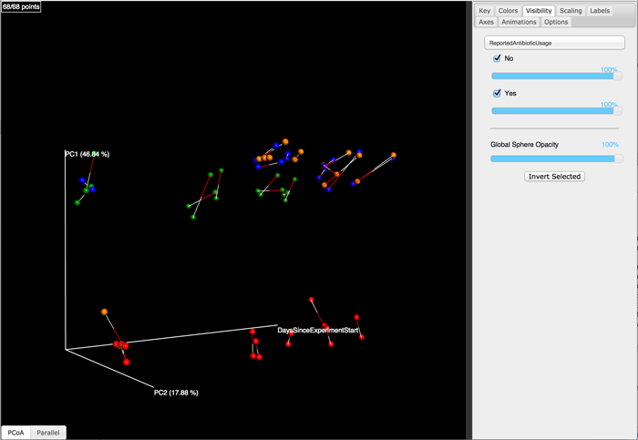
Finally, we’ll generate a Procrustes plot. This plot will include an explicit time axis because we’re passing --custom_axes DaysSinceExperimentStart, but this is not required (it helps with interpretation for this particular data set).

make_emperor.py -c -i procrustes_results/ -o procrustes_results/plots/ -m illumina/map.tsv --custom_axes DaysSinceExperimentStart

There will now be several results of interest. For the Procrustes analysis you can find the statistical results in procrustes_results/procrustes_results.txt and you can view the Procrustes plot by opening procrustes_results/plots/index.html in a web browser. You should see a plot that looks like the following:

Comparing data sets with different sample ids

In the example provided here, we have the same samples in our two principal coordinate matrices. If that is not the case for your study, you’ll need to pass a sample id mapping file, which is different from a QIIME metadata mapping file. For a description of this file format, see Sample id map.